arduino_waveform

The Arduino is an amazing platform for all kinds of projects, but when it comes to generating sound, many users struggle to get beyond simple beeps. With a deeper understanding of the hardware, you can use Arduino to generate any waveform you can imagine, and manipulate it in real time.

Project Steps

Basic Sound Output

“Bit banging” is the most basic method of producing sound from an Arduino. Just connect a digital output pin to a small speaker and then rapidly and repeatedly flip the pin between high and low. This is how the Arduino’s tone() statement works. The output pins can even drive a small (4cm or less) 8-ohm speaker connected directly between the pin and ground without any amplification.

Figure A
Figure A

Cycling the pin once from low to high and back again creates a single square wave (Figure A). Time spent in the high state is called mark time and time spent low, space time. Varying the ratio between mark and space times, aka the duty cycle, without changing the frequency of the wave, will change the quality or “timbre” of the sound.

Figure B
Figure B

The Arduino’s analogWrite() function, which outputs a square wave at a fixed frequency of 490Hz, is handy to illustrate the concept. Connect your speaker to pin D9 and ground (Figure B) and run this sketch:

void setup() {
  pinMode(9,OUTPUT);
}
void loop() {
  for (int i=0; i<255; i++) {
    analogWrite(9,i);
  delay(10);
  }
}

You should hear a tone of constant pitch, with a timbre slowly changing from thin and reedy (mostly space time) to round and fluty (equal mark and space time), and back to thin and reedy again (mostly mark time).

A square wave with a variable duty cycle is properly called a pulse-width modulated (PWM) wave. Altering the duty cycle to change timbre may serve very basic sound functions, but to produce more complex output, you’ll need a more advanced approach.

From Digital to Analog

PWM waves are strictly digital, either high or low. For analog waves, we need to generate voltage levels that lie between these 2 extremes. This is the job of a digital-to-analog converter (DAC).

Figure C
Figure C

There are several types of DAC. The simplest is probably the R-2R ladder (Figure C). In this example, we have 4 digital inputs, marked D0–D3. D0 is the least significant bit and D3 the most significant.

If you set D0 high, its current has to pass through a large resistance of 2R + R + R + R = 5R to reach the output. Some of the current also leaks to ground through the relatively small resistance 2R. Thus a high voltage at D0 produces a much smaller output voltage than a high voltage at D3, which faces a small resistance of only 2R to reach the output, and a large resistance of 5R to leak to ground.

Figure D
Figure D

Setting D0–D3 to binary values from 0000 to 1111 (0–15 decimal), and then back down to 000 in quick succession, ought to output the triangle wave shown in Figure D. To produce other waveforms, in theory, we must simply present the right sequence of binary numbers to D0–D3 at the right rate.

Unfortunately, there are drawbacks to using an R-2R DAC, foremost probably that it requires very precise resistor values to prevent compound errors from adding up and distorting the waveform. The jagged “steps” must also be smoothed, using a low-pass filter, to prevent a discordant metallic sound. Finally, an R-2R DAC uses up more output pins than are strictly necessary.

Though a bit harder to understand, the “1-bit” DAC produces very smooth, high-quality waveforms using just one output pin with a single resistor and capacitor as a filter. It also leaves the Arduino free to do other things while the sound is playing.

One-Bit DAC Theory

If you replace the speaker from the bit-banging sketch with an LED, you’ll see it increase in brightness as the duty cycle increases from 0 to 100%. Between these 2 extremes, the LED is really flashing at around 490Hz, but we see these flashes as a continuous brightness.

Figure E
Figure E

This “smoothing” phenomenon is called “persistence of vision,” and it can be thought of as a visual analogy to the low-pass filter circuit shown in Figure E. You can use this filter to smooth the output from a 1-bit DAC.

The mark time of the incoming PWM wave determines the voltage at Vout from moment to moment. For example, a mark/space ratio of 50:50 outputs 50% of the high voltage of the incoming signal, a 75:25 ratio outputs 75% of that voltage, and so on. An Arduino’s digital pins produce a high of 5V, so a 50% duty cycle, for example, would give 2.5V at Vout.

An LED subjected to “bit banging” in place of the speaker will steadily increase in brightness.

For best sound quality, the frequency of the PWM signal should be as high as possible. Luckily, the Arduino can produce fast PWM waves up to 62.5KHz. The hardware also provides a handy mechanism for updating the mark time from a lookup table at absolutely regular intervals, while leaving the Arduino free to do other things.

The Arduino 1-Bit DAC

The ATmega328 chip at the heart of the Arduino Nano 3 contains 3 hardware timers. Each timer includes a counter that increments at each clock tick, automatically overflowing back to 0 at the end of its range. The counters are named TCNTn, where n is the number of the timer in question.

Timer0 and timer2 are 8-bit timers, so TCNT0 and TCNT2 repeatedly count from 0 to 255. Timer1 is a 16-bit timer, so TCNT1 repeatedly counts from 0 to 65535, and can also be made to work in 8-bit mode. In fact, each timer has a few different modes. The one we need is called “fast PWM,” which is only available on timer1.

In this mode, whenever TCNT1 overflows to zero, the output goes high to mark the start of the next cycle. To set the mark time, timer1 contains a register called OCR1A. When TCNT1 has counted up to the value stored in OCR1A, the output goes low, ending the cycle’s mark time and beginning its space time. TCNT1 keeps on incrementing until it overflows, and the process begins again.

Figure F
Figure F

This process is represented graphically in Figure F. The higher we set OCR1A, the longer the mark time of the PWM output, and the higher the voltage at Vout. By updating OCR1A at regular intervals from a pre-calculated lookup table, we can generate any waveform we like.

Basic Wave Table Playback

Listing 1 (download Listings 1–6 as a .zip file) contains a sketch that uses a lookup table, fast PWM mode, and a 1-bit DAC to generate a sine wave.

LISTING 1

#include <avr/interrupt.h> // Use timer interrupt library

/******** Sine wave parameters ********/
#define PI2 6.283185 // 2*PI saves calculation later
#define AMP 127 // Scaling factor for sine wave
#define OFFSET 128 // Offset shifts wave to all >0 values

/******** Lookup table ********/
#define LENGTH 256 // Length of the wave lookup table
byte wave[LENGTH]; // Storage for waveform

void setup() {

/* Populate the waveform table with a sine wave */
for (int i=0; i<LENGTH; i++) { // Step across wave table
   float v = (AMP*sin((PI2/LENGTH)*i)); // Compute value
   wave[i] = int(v+OFFSET); // Store value as integer
 }

/****Set timer1 for 8-bit fast PWM output ****/
 pinMode(9, OUTPUT); // Make timer’s PWM pin an output
 TCCR1B = (1 << CS10); // Set prescaler to full 16MHz
 TCCR1A |= (1 << COM1A1); // Pin low when TCNT1=OCR1A
 TCCR1A |= (1 << WGM10); // Use 8-bit fast PWM mode
 TCCR1B |= (1 << WGM12);

/******** Set up timer2 to call ISR ********/
 TCCR2A = 0; // No options in control register A
 TCCR2B = (1 << CS21); // Set prescaler to divide by 8
 TIMSK2 = (1 << OCIE2A); // Call ISR when TCNT2 = OCRA2
 OCR2A = 32; // Set frequency of generated wave
 sei(); // Enable interrupts to generate waveform!
}

void loop() { // Nothing to do!
}

/******** Called every time TCNT2 = OCR2A ********/
ISR(TIMER2_COMPA_vect) { // Called when TCNT2 == OCR2A
 static byte index=0; // Points to each table entry
 OCR1AL = wave[index++]; // Update the PWM output
 asm(“NOP;NOP”); // Fine tuning
 TCNT2 = 6; // Timing to compensate for ISR run time
}

First we calculate the waveform and store it in an array as a series of bytes. These will be loaded directly into OCR1A at the appropriate time. We then start timer1 generating a fast PWM wave. Because timer1 is 16-bit by default, we also have to set it to 8-bit mode.

We use timer2 to regularly interrupt the CPU and call a special function to load OCR1A with the next value in the waveform. This function is called an interrupt service routine (ISR), and is called by timer2 whenever TCNT2 becomes equal to OCR2A. The ISR itself is written just like any other function, except that it has no return type.

The Arduino Nano’s system clock runs at 16MHz, which will cause timer2 to call the ISR far too quickly. We must slow it down by engaging the “prescaler” hardware, which divides the frequency of system clock pulses before letting them increment TCNT2. We’ll set the prescaler to divide by 8, which makes TCNT2 update at 2MHz.

To control the frequency of the generated waveform, we simply set OCR2A. To calculate the frequency of the resulting wave, divide the rate at which TCNT2 is updated (2MHz) by the value of OCR2A, and divide the result by the length of the lookup table. Setting OCR2A to 128, for example, gives a frequency of:

Arduino-synth-equation

which is roughly the B that’s 2 octaves below middle C. Here’s a table of values giving standard musical notes.

The ISR takes some time to run, for which we compensate by setting TCNT2 to 6, rather than 0, just before returning. To further tighten the timing, I’ve added the instruction asm(“NOP;NOP”), executing 2 “no operation” instructions using one clock cycle each.

Sound synth_figF

Figure G
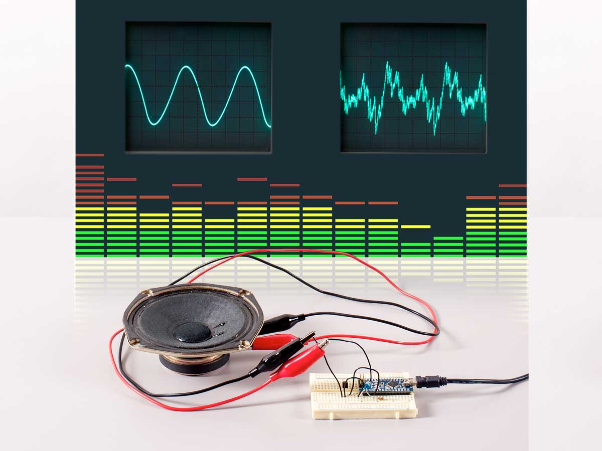
Figure G

Run the sketch and connect a resistor and capacitor (Figure G). You should see a smooth sine wave on connecting an oscilloscope to Vout. If you want to hear the output through a small speaker, add a transistor to boost the signal (Figure H, below).

Sound synth_figJ

Figure H
Figure H

Programming Simple Waves

Once you know how to “play” a wave from a lookup table, creating any sound you want is as easy as storing the right values in the table beforehand. Your only limits are the Arduino’s relatively low speed and memory capacity.

Listing 2 contains a waveform() function to prepopulate the table with simple waveforms: SQUARESINETRIANGLERAMP, and RANDOM. Play them to see how they sound (below).

A SQUARE waveform can have a timbre ranging from round and fluty to thin and reedy, depending on its duty cycle. From our initial experiments with bit banging, we already know that a 50% duty cycle gives a flute-like sound.
A SINE waveform consists of a smoothly oscillating curved signal representing the graph of the trigonometric function. It produces a clear, glassy tone that sounds very much like a tuning fork.
A TRIANGLE waveform looks a little like a sine wave with sharp points and straight lines, or 2 ramp waveforms squashed back to back. It has a more interesting, rounded sound than a sine wave, a little like an oboe.
A RAMP waveform consists of steadily increasing values, starting at zero. At the end of the waveform the value suddenly drops to zero again to begin the next cycle. The result is a sound that’s bright and brassy.
A RANDOM waveform can sound like anything, in theory, but usually sounds like noisy static. The Arduino produces only pseudorandom numbers, so a particular randomSeed() value always gives the same “random” waveform.

The RANDOM function just fills the table with pseudorandom integers based on a seed value. Changing the seed value using the randomSeed() function allows us to generate different pseudorandom sequences and see what they sound like. Some sound thin and weedy, others more organic. These random waveforms are interesting but noisy. We need a better way of shaping complex waves.

Additive Synthesis

In the 19th century, Joseph Fourier showed that we can reproduce, or synthesize, any waveform by combining enough sine waves of different amplitudes and frequencies. These sine waves are called partials or harmonics. The lowest-frequency harmonic is called the first harmonic or fundamental. The process of combining harmonics to create new waveforms is called additive synthesis.

Given a complex wave, we can synthesize it roughly by combining a small number of harmonics. The more harmonics we include, the more accurate our synthesis.

Professional additive synthesizers can combine over 100 harmonics this way, and adjust their amplitudes in real time to create dramatic timbre changes. This is beyond the power of Arduino, but we can still do enough to load our wave table with interesting sounds.

Figure J—Adding the third harmonic creates a waveform that has a distinctly square look and sound, though still very rounded.

Consider the loop in Listing 1 that calculates a sine wave. Call that the fundamental. To add, say, the third harmonic at 1/4 amplitude (Figure J), we add a new step:

for (int i=0; i<LENGTH; i++) { //
Step across table
  float v = (AMP*sin((PI2/LENGTH)*i)); // Fundamental
  v += (AMP/4*sin((PI2/LENGTH)*(i*3))); // New step
  wave[i]=int(v+OFFSET); // Store as integer
  }

In this new step, we multiply the loop counter by 3 to generate the third harmonic, and divide by an “attenuation” factor of 4 to reduce its amplitude.

Listing 3 (available at makezine.com/35) contains a general version of this function. It includes 2 arrays listing the harmonics we want to combine (including 1, the fundamental) and their attenuation factors.

Figure K—Adding the first 8 odd harmonics gives a fairly good approximation of a square wave. Individual sine waves appear as little ripples. Combining more partials would reduce the size of these ripples.

To change the timbre of the sound loaded into the lookup table, we just alter the values in the 2 arrays. A zero attenuation means the corresponding harmonic is ignored. The arrays in Listing 3, as written, produce a fairly good square wave (Figure K). Experiment with the arrays and see what sounds result.

Morphing Waveforms

Professional synthesizers contain circuits or programs to “filter” sound for special effects. For instance, most have a low-pass filter (LPF) that gives a certain “waa” to the start and “yeow” to the end of sounds. Basically, an LPF gradually filters out the higher partials. Computationally, true filtering is too much for Arduino, but there are things we can do to the sound, while it’s playing, to give similar effects.

Listing 4 includes a function that compares each value in the wave table to a corresponding value in a second “filter” table. When the values differ, the function nudges the wave value toward the filter value, slowly “morphing” the sound as it plays.

Using a sine wave as the “filter” approximates true low-pass filtering. The harmonics are gradually removed, adding an “oww” to the end. If we morph the other way — by loading the wave table with a sine wave and the “filter” table with a more complex wave — we add a “waa” quality to the start. You can load the 2 tables with any waves you like.

Creating Notes

What if we want to make a sound fade away, like a real instrument that’s been plucked, strummed, or struck?

Listing 5 contains a function that “decays” the sound to silence by steadily nudging the wave table values back toward a flat line. It steps across the wave table, checking each value — if it’s more than 127, it’s decremented, and if less, incremented. The rate of decay is governed by the delay() function, called at the end of each sweep across the table.

Once the wave is “squashed,” running the ISR just ties up the CPU without making sound; the cli() function clears the interrupt flag set in setup by sei(), switching it off.

Using Program Memory

The Arduino’s Atmel processor is based on the “Harvard” architecture, which separates program memory from variable memory, which in turn is split into volatile and nonvolatile areas. The Nano only has 2KB of variable space, but a (relatively) whopping 30KB, or so, of usable program space.

It is possible to store wave data in this space, greatly expanding our repertoire of playable sounds. Data stored in program space is read only, but we can store a lot of it and load it into RAM to manipulate during playback.

Listing 6 demonstrates this technique, loading a sine wave from an array stored in program space into the wave table. We must include the pgmspace.h library at the top of the sketch and use the keyword PROGMEM in our array declaration:

prog_char ref[256] PROGMEM = {128,131,134,…};

Prog_char is defined in pgmspace.h and is the same as the familiar “byte” data type.

If we try to access the ref[] array normally, the program will look in variable space. We must use the built-in function pgm_read_byte instead. It takes as an argument the address of the array you want to access, plus an offset pointing to individual array entries.

If you want to store more than one waveform this way, you can access the array in pgm_read_byte like a normal two-dimensional array. If the array has, say, dimensions of [10][256], you’d use pgm_read_byte(&ref[4][i]) in the loop to access waveform 4. Don’t forget the & sign before the name of the array!

GENERATING WAVE TABLE DATA

To read wave table data from program memory, you have to hard-code it into your sketch and can’t generate it during runtime. So where does it come from? One method is to generate wave table data in a spreadsheet and paste it into your sketch. We’ve created a spreadsheet that will allow you to generate wave tables using additive synthesis, to see the shape of the resulting waves, and to copy out raw wave table data to insert into your sketch. Download it here.

Going Further

Audio feedback is an important way of indicating conditions inside a running program, such as errors, key presses, and sensor events.

Sounds produced by your Arduino can be recorded into and manipulated by a software sampler package and used in music projects

Morphing between stored waveforms, either in sequence, randomly, or under the influence of performance parameters, could be useful in interactive art installations.

If we upgrade to the Arduino Due, things get really exciting. At 84MHz, the Due is more than 5 times faster than the Nano and can handle many more and higher-frequency partials in fast PWM mode. In theory, the Due could even calculate partials in real time, creating a true additive synthesis engine.