In the early 1950s, aircraft development created an urgent need for simulations, and analog computers were ideally suited to run flight simulators.
Digital computers barely existed in those days, but aircraft dynamics could be modeled by the flow of electric current through potentiometers, amplifiers, and capacitors. Such circuits were analogous to the real world, and so they became known as analog computers.


You could describe almost all aspects of aircraft performance with differential equations, and the terms in these equations were represented by chaining together analog modules using patch cords on a plug board. This created a formidable tangle of wires, but once you got it right, the output on an oscilloscope screen was immediate, with no processing or programming necessary. Figure  A shows an installation at the NASA Glenn Research Center in 1956. (Note the plug boards.)
As late as 1963, analog computation was still being used to create a cockpit simulation of a space vehicle docking in orbit. But microchips promised greater accuracy with much less maintenance, and they became less expensive. By the mid-1970s, analog was obsolete.
Or was it?
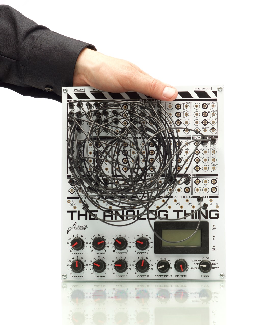
In 2020, Professor Doctor Bernd Ulmann cofounded Anabrid GmbH in Frankfurt, Germany, to develop chip-based analog computers. The company also introduced an educational product named The Analog Thing , abbreviated as THAT. Digital computers running complex simulations had become increasingly power-hungry and plagued with problems such as heat dissipation, prompting Ulmann and his colleagues to foresee a new role for analog.

THAT is now available to buyers in the United States for less than $350, including shipping (see Figure B  ). “Our goal is to bring the idea of analog computing back to the world,” Ulmann states. “We have hobbyists, musicians (controlling analog synthesizers), many students, sometimes large companies. There is a THAT group at Facebook where users ask questions and post their computer setups. They have simulated events such as a bungee jump with a quite realistic rubber rope, and gravitational waves, neurons, many more.”
Ulmann claims that seriously challenging tasks, such as creating an epidemiological model, “can be done easily” with THAT. And if a problem gets too big, one THAT can be daisy-chained with another. The key is to express a phenomenon as a series of mathematical terms, each represented by a computing element. Connect them together, and the input flows directly to the output.
THAT is open-source, because Ulmann wants to encourage innovation and analog literacy, although he sees THAT being integrated with digital systems. “We have a little application example showing how an Arduino can be used as the digital part of a hybrid computer setup,” he says. “The community has already come up with a data logger and an Arduino-based oscilloscope.” And to spread the gospel, he has written a book titled Analog and Hybrid Computer Programming.
Meanwhile, you can build your own basic analog computing device for around $5 (see the following project) to understand how they work.
The best way to understand an analog computer is to build one, which you can do on a very limited scale using only three potentiometers and a multimeter. This little project is derived from the EF-140 kit marketed in 1961 by General Electric (see Figure  C). Because analog computers always seem to have names consisting of acronyms, I’m calling my version EASY, for Elementary Analog SYstem.

TIME REQUIRED: 1-2 hours
DIFFICULTY: Easy
COST: $5-15


The schematic for EASY is shown in Figure  D, and indeed it’s so easy, you can assemble it with alligator jumper wires, as in Figure
  E. You do need to put in a bit of extra work, though, by mounting pointers on the potentiometers and adding dials like the one in Figure F
 . Put a blank circle of paper on the front of each potentiometer and use your meter to measure the resistance between the wiper and the left terminal, while you turn the shaft and mark 10 equal intervals between the ends of the range.
How do you use EASY? Well, it’s — simple. Here’s a quick demo for doing multiplication: First move the wiper of Pot A to a position such as 0.3 on the dial. If letter V represents the voltage of your supply, the wiper of Pot A will tap a voltage of 0.3 * V . This is passed along to the top of Pot B, so if you set its wiper to a position labeled 0.7, the voltage there will be 0.7 * 0.3 * V — right?

Turn Pot C till there is no difference in voltage between points VA and VB in the schematic, measured with your meter (although I used a $9 galvanometer to get that authentic analog look, as in Figure G  ). Pot C now points to 0.21 on its scale. Yes, you just proved that 0.7 * 0.3 = 0.21 (approximately). The answer won’t be precise, because Pot B steals a bit of current from Pot A. To minimize this, I used a 100K value for Pot B while Pot A is only 1K.
You can learn some general lessons from your EASY demo. Analog components must be accurately made, inputs are prone to error, results are always approximate, and if you have more than a couple of modules in your computer, voltage amplifiers will be necessary.
Still, the output is immediate and your three-pot computer is versatile. You can use it for division: Set a number on Pot C, divide it by a number on Pot B, and read the result off Pot A when you zero the voltage between VA and VB. You can even do a square root: Set a number on Pot C, then turn pots A and B till their values are the same while the voltage between VA and VB is zero. This is another feature of analog computation: Changing the sequence of operations enables you to process different formulae.
If you want to know how to build serious analog modules, you can find basic circuits in “A Practical Approach to Analog Computers (pdf) ,” archived by The Analog Museum.

Or, you can hunt for vintage kits such as the Heathkit ES-400 (shown in Figure  H), which used 73 vacuum tubes for its op-amps. Supposedly, it weighed 168lbs, so if you find one on eBay, don’t expect free shipping.